Widespread across Europe, indicating active transmission
Data Source: ADIS (Animal Disease Information System) Weekly Notification Created: November 14, 2025
Header image photo credit: Cynthia Goldsmith Content Providers: CDC/ Courtesy of Cynthia Goldsmith; Jacqueline Katz; Sherif R. Zaki
This media comes from the Centers for Disease Control and Prevention’s Public Health Image Library (PHIL), with identification number #1841
The big challenge: Keeping sows healthy and productive – Part 1 General aspects to be observed
Dr. Inge Heinzl – Editor of EW Nutrition and
Dr. Merideth Parke – Global Application Manager for Swine, EW Nutrition
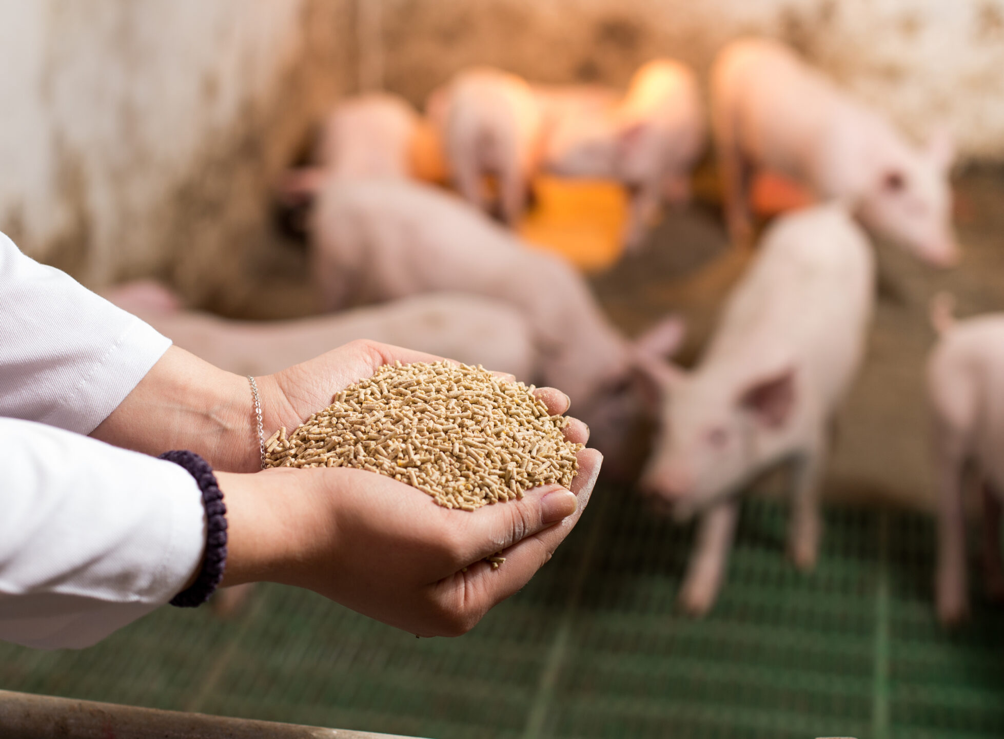
Sow mortality critically impacts herd performance and efficiency in modern pig production. Keeping the sows healthy is, therefore, the best strategy to keep them alive and productive and the farm’s profitability high.
Rising mortality rates are alarming
In recent years, sow mortality has increased across pig-raising regions in many countries. Eckberg’s (2022) findings from the MetaFarms Ag Platform (including farms across the United States, Canada, Australia, and the Philippines) determined an increase of 66.2% between 2012 and 2021.
Figure 1: Sow mortality rates from 2012 to 2021 (Eckberg, 2022)
What can be done to decrease mortality rates?
Several measures can be taken to reach a particular stock of healthy and high-performing sows. In the following, the main remedial actions will be explained.
1. Determination of the cause of death
If a sow is dead, it must first be clarified why it has died. If the sow is culled, the reason for this decision is usually apparent. If the sow suddenly dies, investigations, including a thorough postmortem, are extremely valuable to determine the cause of death. Kikuti et al. (2022) provided a collection of the most-occurring causes of death in the years 2009 to 2018. As often, no necropsy is conducted, and the causes of death remain unclear, as shown by the high numbers of “other”. Locomotory (e.g., lameness) and reproductive (e.g., prolapse, endotoxemic shock from retained fetuses) incidents account for approximately half of the recorded sow mortalities (Kikuti et al., 2022), especially during the first three parities. (Marco, 2024).
Figure 2: Removal reasons and their frequency from 2009 to 2018 (Kikuti et al., 2022)
Evaluating detailed breeding history together with the cause of death will provide perspective and assist veterinary, nutritionist, and husbandry teams with interventions to prevent similar events and early sow mortality.
Selection of the gilts
After selecting the best genetics and rearing the gilts under the best conditions, further selection must focus on physical traits such as structure, weight, height, leg, and hoof integrity.
Additionally, as we have more and more group housing for sows, the selection for stress resilience can positively impact piglet performance (Luttmann and Ernst, 2024). The following table compares stress-resilient and stress-vulnerable sows concerning piglet performance and shows the piglets of the vulnerable sows with worse performance.
Least square means and standard error of stress resilient (SR) and stress vulnerable (SV) for each trait; significance threshold of p<0.05 with * indicating 0.01<p<0.05, ** indicating 0.001<p<0.01
How to manage the gilts best
The management of the gilts must consider the following:
Age at first estrus should be <195 days:
Gilts having their first estrus earlier show higher daily gain and usually higher lifetime productivity. In a study conducted by Roongsitthichai et al. (2013), sows culled at parity 0 or 1 exhibited first estrus at 204.4±0.7 days of age, while those culled at parity ≥5 exhibited first estrus at 198.9±2.1 days of age (P=0.015).
Age at first breeding should lay between 200 and 225 days:
If the sows are bred at a higher age, they have the risk of being overweight, leading to smaller second-parity litters, longer wean-to-service intervals, and shorter production life.
The body weight at first mating should be between 135 and 160 kg:
To reach this target within 200-225 days, the gilts must have 600-800 g of average daily gain. Breeding underweight gilts reduces first-litter size and lactation performance. Overweight gilts (>160 kg) face higher maintenance costs and locomotion issues.
The number of estruses at first mating should be 2 or 3:
Accurately track estrus and breed on the second estrus. Research shows that delaying breeding to the second estrus positively affects litter size. Only delay breeding to the third estrus to meet minimum weight targets.
Housing
Gestating sows are more and more held in groups. Understanding the process of group housing is essential for success. The following graphic shows factors impacting successful grouping.
Figure 3: Factors influencing group housing
If the groups are not well-established yet, the stress levels among sows are higher, leading to
More leg injuries due to aggressive behavior or fighting for resources
Higher rates of abortions and returns to service
Reduced sow performance, including decreased productivity, lower milk yield, and poor piglet growth due to compromised immune function and overall health
To mitigate stress in group housing, it is crucial to implement proper group management practices, which include gradual introductions, maintaining stable social structures, and ensuring adequate space and resources. This helps promote a calmer environment, improving animal welfare and herd performance.
Responsible on-farm pig care
Caregivers must be well-trained and equipped to provide high-quality care. Insufficient or unskilled pig caregivers can significantly affect the growth and development of prospective replacement gilts, ultimately influencing their suitability for the breeding herd:
Growth Rates: Suboptimal nutrition and health management result in slower growth rates and poor body condition.
Health Issues: Unskilled handling may increase the risk of disease transmission, injuries, and stress, all of which can adversely affect growth and overall development.
Behavioral Problems: Poorly managed environments can increase aggression and competition among animals, hindering growth and health.
Selection Criteria: Ineffective growth and health monitoring can result in misjudging the potential of gilts, leading to the selection of less suitable candidates for the breeding herd.
Table 2: Influence of handling on growth performance and corticosteroid concentration of female grower pigs from 7-13 weeks of age (Hemsworth et al., 1987)
Unpleasant
Pleasant
Inconsistent
Minimal
ADG (g)
404a
455b
420ab
4.58b
FCR (F:G)
2.62b
2.46a
2.56b
2.42a
Corticosteroid conc (ng/mL)
2.5a
1.6b
2.6a
1.7b
Responsible on-farm pig care is crucial to keep sows healthy and performing. Poor sow observations (e.g., failure to identify stressed, anorexic, or heat-stressed sows) or inappropriate farrowing interventions can directly influence sow health and potentially reduce subsequent performance or mortality. On the contrary, rapid and proactive identification of sows needing intervention can save many animals that would otherwise die or need to be culled.
Keeping sows healthy and performing is manageable
The maintenance of sows’ health is a challenge but manageable. Observing all the points mentioned, from selecting the right genetics over rearing the piglets under the best conditions to managing the young gilts, can help prevent disease and performance drops. For all these tasks, farmers and farm workers who do their jobs responsibly and passionately are needed. The following article will show nutritional interventions supporting the sow’s gut and overall health.
Hemsworth, P.H., J.L. Barnett, and C. Hansen. “The Influence of Inconsistent Handling by Humans on the Behaviour, Growth and Corticosteroids of Young Pigs.” Applied Animal Behaviour Science 17, no. 3–4 (June 1987): 245–52. https://doi.org/10.1016/0168-1591(87)90149-3.
Kikuti, Mariana, Guilherme Milanez Preis, John Deen, Juan Carlos Pinilla, and Cesar A. Corzo. “Sow Mortality in a Pig Production System in the Midwestern USA: Reasons for Removal and Factors Associated with Increased Mortality.” Veterinary Record 192, no. 7 (December 22, 2022). https://doi.org/10.1002/vetr.2539.
Roongsitthichai, A., P. Cheuchuchart, S. Chatwijitkul, O. Chantarothai, and P. Tummaruk. “Influence of Age at First Estrus, Body Weight, and Average Daily Gain of Replacement Gilts on Their Subsequent Reproductive Performance as Sows.” Livestock Science 151, no. 2–3 (February 2013): 238–45. https://doi.org/10.1016/j.livsci.2012.11.004.
Immunoglobulins – Novel solutions for swine health
Conference Report
Unlike humans and most mammals, piglets do not receive any maternal immunoglobulins (antibodies) via the placenta. Therefore, it is vital for piglets to receive maternal antibodies via the colostrum within 24 hours of birth. Otherwise, they are more vulnerable to illnesses in their early stages of life. In situations where piglets do not receive enough colostrum, such as due to large litter sizes or weak sows following a prolonged farrowing — supplemental colostrum or IgY products can provide essential immune protection.
In the following, Dr. Shofiqur Rahman describes the innovative role of IgY – yolk immunoglobulins in enhancing swine health.
IgY – modes of action
IgY is an antibody found in egg yolk. It is an entirely natural product; each egg contains approximately 100 mg of IgY. These egg-derived antibodies primarily function in the gut through several mechanisms:
Adherence inhibition – IgY antibodies bind to specific structures on the surface of pathogens (such as fimbriae, flagella, and lipopolysaccharides), preventing them from adhering to the intestinal mucosa and blocking the initial stages of infection. This is particularly significant for enterotoxigenic E. coli (ETEC), which causes piglet diarrhea by attaching to intestinal cells.
Neutralization – IgY can neutralize toxins produced by pathogens, preventing them from exerting harmful effects on host cells.
Agglutination – IgY promotes the clumping of pathogens by binding them together, effectively immobilizing them, and facilitating their removal from the animal’s gut.
Cell damage – IgY can damage the integrity of bacterial cell walls leading to cell lysis and reduced bacterial viability.
Furthermore, because these pathogens are bound in complexes with IgY and eliminated through feces in an inactivated form, IgY helps prevent environmental re-infection through manure.
IgY and IgG – functional differences
Both IgY and Immunoglobulin G (IgG) (IgG, the most abundant immunoglobulin in mammals) are antibodies. They, however, exhibit significant differences due to their distinct structural characteristics. “IgY, for instance, does not activate the complement system, a key function of IgG that enhances immune responses against infections. Additionally, IgY promotes more rapid phagocytosis and reduces inflammation compared to IgG. These effects contribute to energy conservation, thereby facilitating improved animal growth performance,” he explained.
IgY is more hydrophobic than IgG, which increases its stability and resistance to proteolytic degradation. This property is beneficial for maintaining its functionality in the gastrointestinal tract.
Production and quality control
IgY develops in hens in response to the pathogens they encounter, regardless of their relevance to the hens themselves. For instance, hens immunized with an infectious pathogen affecting pigs can produce IgY, effectively preventing the disease caused by that pathogen.
There are different methods of IgY production. One possibility is to hyperimmunize the hens simultaneously with multiple antigens. This method seems convenient, but it does not produce products with standardized levels of immunoglobulins for each antigen.
Another approach involves immunizing different groups of hens, each with a single antigen (e.g., transmissible gastroenteritis virus, rotavirus, E. coli) that commonly challenges piglets during the first weeks of life. The immunoglobulin content is then quantified, and the resulting egg powders are spray-dried, pasteurized, and mixed. This process yields an IgY product with standardized amounts of specific immunoglobulins that exhibit high affinity for the target pathogens.
One health application in swine
“The benefits of IgY have been demonstrated through extensive trials and commercial experiences, highlighting its potential for various applications not only in swine but also in other animals and humans,” said Dr. Rahman.
Due to concerns about antibiotic resistance, regulatory and consumer scrutiny increased over the use of in-feed antibiotics. IgY can serve as an effective and natural alternative for improving overall gut health, reducing the incidence and severity of diarrhea, reducing morbidity during the critical pre- and post-weaning periods, and, thereby, increasing performance.
Unlike antibiotics, which can indiscriminately kill both harmful and beneficial bacteria, IgY selectively targets specific pathogens. This selective action helps maintain a balanced gut microbiome, which is crucial for overall health and digestion in piglets. Disruption of the gut microbiota by antibiotics can lead to issues such as antibiotic-associated diarrhea and increased susceptibility to opportunistic infections due to the loss of beneficial microbes.
In contrast to antibiotics, IgY targets multiple antigenic sites on pathogens, requiring various genes for their protection, thereby avoiding resistance issues among pathogenic microorganisms. Additionally, IgY is effective not only against bacteria but also demonstrates significant efficacy against viruses and coccidia.
Conclusion
Dr. Rahman concluded that “the use of IgY as a passive immunization strategy, incorporated into a holistic approach to reducing piglet diarrhea, offers a safe and natural alternative to traditional antibiotics, particularly in the light of rising antibiotic resistance and the need for effective treatments also for viral diseases.”
EW Nutrition’s Swine Academy took place in Ho Chi Minh City and Bangkok in October 2024. Dr. Shofiqur Rahman, Senior Researcher at the Immunology Research Institute Gifu (IRIG) in Japan was one of the highly experienced speakers of EW Nutrition. Originally a microbiologist, Dr. Rahman focuses on researching and developing IgY products for Human, Animal, Pet, Fish, Plant, and Environmental health.
The Science Behind Phytogenics
Conference Report
Essential oils, secondary plant compounds, phytogenics – all these expressions can be found in the context of animal feed. In the following, Dr. Sabiha Kadari, Regional Technical Director Southeast Asia/Pacific at EW Nutrition, will show the difference between essential oils and phytomolecules and the science behind phytogenics.
Essential oils and phytomolecules– not the same
Let us first show what are essential oils using the example of oregano oil. Essential oils are extracted from plants and unpurified mixes of different phytomolecules. The raw oregano oil extract contains carvacrol, thymol, P-cymene, and several other phytomolecules. The concentration and composition of these phytomolecules can vary significantly, depending on factors such as geographical origin, seasonal variations, plant part, plant growth stage and harvest time, extraction methods, and post-harvest processing. As a result, there can be significant batch-to-batch variations, resulting in differences in animal performance. Furthermore, there is the potential for the presence of undesirable contaminants.
In contrast, phytomolecules are the active ingredients in essential oils or other plant materials. They are clearly defined as one active compound (IUPAC name/CAS number) by their unique chemical structures, such as carvacrol. By focusing on specific active compounds, standardized products don’t have batch-to-batch variation, enhancing consistent animal performance.
Stringent screening processes
To yield the best phytogenic formulations for animal production, a rigorous screening process is required:
The initial screening process consists of ensuring the bioactives are generally recognized as safe (GRAS) by the US Department of Agriculture and approved by the European Food Safety Authority (EFSA). This step is crucial to ensure that any compounds used in formulations do not pose health risks to animals or humans.
In addition to being selected for their chemical-physical properties, which play a significant role in determining how well the phytogenics will perform in various applications, and a thorough cost-benefit analysis, the phytogenics are mapped for their following biological activities.
Antioxidant
Phytomolecules exert their antioxidant effects through various mechanisms, including scavenging free radicals. The ORAC (Oxygen Radical Absorbance Capacity) test is widely regarded as a gold standard for measuring the antioxidant potential of phytomolecules. It quantitatively assesses the ability of compounds to scavenge free radicals, providing a reliable comparison against a known standard, specifically Trolox, a vitamin E analog. Trolox has well-documented antioxidant properties, making it a reliable benchmark for evaluating the effectiveness of other antioxidants.
Antimicrobial
Incorporating a comprehensive approach to testing the antibacterial properties of phytogenics is essential for developing effective feed additives. The antibacterial properties should not only be tested against harmful enteropathogenic bacteria, such as Clostridium perfringens, E. coli, and Salmonella. It should also be evaluated if beneficial species such as Lactobacilli, the proliferation of which is wanted, are preserved.
By evaluating both pathogenic and beneficial bacteria, researchers can ensure that phytogenic formulations support optimal gut health and reduce the reliance on antibiotics.
Anti-inflammatory
Anti-inflammatory properties also help to modulate the gut-associated immune system and mitigate excessive immune response so that animals can allocate more energy towards growth and production. This shift is vital for optimizing feed conversion ratios and overall performance.
Dr. Kadari noted that “EW Nutrition uses nuclear factor kappa beta (NFkß), which regulates the expression of various pro-inflammatory cytokines, and interleukin 6 (pro-inflammatory) and 10 (anti-inflammatory) cytokines as biomarkers, for measuring anti-inflammatory activity. A reduction in NFkß and the ratio of IL-6/ IL-10 indicates a decrease in inflammatory response.”
Anti-conjugation
Conjugation is a common mechanism of horizontal gene transfer that is instrumental in spreading antibiotic resistance between bacteria. “Most resistance genes are found on mobile genetic elements named plasmids and primarily spread by conjugation,” explained Dr. Kadari.
Cell stress of bacteria modulates the conjugation frequency. Among these stressors are antimicrobial phytogenics. The goal is to keep the conjugation frequency below the one that could occur under unchallenged conditions.
Figure 1: High throughput screening allows EW Nutrition researchers to quickly conduct millions of chemical, genetic, or pharmacological tests
Delivery mechanism
Lastly, to optimize the benefit of the selected phytogenics and deliver consistent results, the substances must be protected by, e.g., encapsulation to ensure homogenous distribution in feed and thermostability in pelleted feed. A special delivery system provides for the targeted release of the active ingredients within the organism, specifically ensuring that these compounds are effectively utilized within the body rather than eliminated through the feces. This is crucial for optimizing their benefits in animal production.
Phytomolecules are an essential support in antibiotic reduction
“Phytogenics are increasingly recognized as effective alternatives in antimicrobial reduction programs. The combination of stringent screening processes alongside rigorous in vitro and in vivo testing is essential for ensuring that phytogenics deliver optimal and consistent performance in animal production,” noted Dr. Kadari.
EW Nutrition’s Swine Academies took place in Ho Chi Minh City and Bangkok in October 2024. Dr. Sabiha Kadari, Regional Technical Director at EW Nutrition SEAP, was one of the highly experienced speakers of EW Nutrition. With expertise in feed cost optimization, feed additive management, audits, and lab support, she provides customized technical solutions and troubleshooting challenges for customers.
Consequences of genetic improvements and nutrient quality on production performance in swine
Conference Report
Achieving high performance and superior meat quality with preferably low investment – and here, we speak about feed costs, which account for up to 70% of the total costs – is a considerable challenge for pig producers. The following will focus on the effects of genetic enhancements and nutrient quality on overall pig performance.
Effect of body weight and gender on protein deposition
Based on Schothorst Feed Research recommendations for tailoring nutritional strategies to enhance feed efficiency and overall productivity, the following facts must be considered:
Castrates, boars, and gilts have significantly different nutritional requirements due to variations in growth rates, body composition, and hormonal influences. For instance, testosterone significantly impacts muscle development and protein metabolism, increasing muscle mass in males. In contrast, ovarian hormones may inhibit muscle protein synthesis in females, contributing to differences in overall protein deposition. Boars, therefore, require higher protein levels to support muscle growth. Castrates typically have a higher FCR compared to gilts and boars due to higher feed intake. Split-sex feeding allows for diet adjustments to optimize growth rates and reduce feed costs per kilogram gained.
Different body weight ranges: because puberty is delayed in modern genetics, we can produce heavier pigs without compromising carcass quality. Given that a finisher pig with 80-120 kg bodyweight consumes about half of the total feed of that pig, Dr. Fledderus concluded that extra profit could be realized with an extra feed phase diet for heavy pigs. Implementing multiple finisher diets can help reduce feed costs by allowing for lower nutrient concentrations, such as reducing the net energy and standardized ileal digestible lysine in later phases, without compromising performance.
Decision-making according to feedstuff prices
Least cost formulation is commonly used by nutritionists to formulate feeds for the lowest costs possible while meeting all nutrient requirements and feedstuff restrictions at the actual market prices of feedstuffs. However, diet optimization is more complex. The real question is, “How do you formulate diets for the lowest cost per kilogram of body weight gain?” You must always consider your specific situation, as economic results vary greatly and depend mainly on the prices of pork and feed and pig growth performance (e.g., feed efficiency, slaughter weight, and lean percentage).
How can you optimize your feeding strategy? Reducing net energy (NE) value will result in more fiber entering the diet. This makes sense if fiber by-products are cheaper than cereals. In contrast, an increase in the NE value will increase the inclusion of high-quality proteins and synthetic amino acids. It will use more energy from fat and less from carbohydrates.
The effects of diet composition on meat quality and fat composition also need to be considered.
How can nutrition improve meat quality?
Nutritional strategies not only improve the sensory attributes of pork but also enhance its shelf life, ultimately leading to higher consumer satisfaction and better marketability. Some of the factors Dr Fledderus considered included:
Improving fat quality
The source of dietary fat significantly impacts the quality of pork fat. Saturated fats tend to produce firmer fat, while unsaturated fats can lead to softer, less stable fat deposits. Diets high in unsaturated fats are more prone to lipid oxidation, negatively affecting shelf life and overall meat quality. The deposition of polyunsaturated fatty acids is only from dietary fat. Saturated fats in pork, partly originates from dietary fat and are also synthesized de novo. So, the amount of polyunsaturated fatty acids in pork depends on the content and composition of dietary fat, which can negatively affect the shelf life and perception of pork meat.
The iodine value (IV) is a measure of the degree of unsaturation in fats. A higher IV indicates a higher proportion of unsaturated fatty acids, leading to softer fat. Pork fat with an IV lower than 70 is considered high quality, as it tends to be firmer and more desirable for processing.
As per the American Oil Chemists Society, IV is calculated as:
Dr. Fledderus concluded that the pigs’ nutritional requirements are dynamic and influenced by factors such as required meat and fat quality, heat stress, slaughter weight, and genetic developments. Tailoring diets based on gender and body weight is crucial for optimizing protein deposition. Accurate information is essential to formulate diets that achieve optimum economic results, not just the least cost.
Continuous monitoring of feedstuff prices and nutritional content allows for timely adjustments in diet formulations, ensuring that producers capitalize on cost-effective ingredients while maintaining nutritional quality.
EW Nutrition’s Swine Academy took place in Ho Chi Minh City and Bangkok in October 2024. Dr. Jan Fledderus, Product Manager and Consultant at the S&C team at Schothorst Feed Research, with a strong focus on continuously improving the price/quality ratio of the diets for a competitive pig sector and one of the founders of the Advanced Feed Package, was a reputable guest speaker in these events.
Recent advances in energy evaluation in pigs
Conference Report
During the recent EW Nutrition Swine Academies in Ho Chi Minh City and Bangkok, Dr. Jan Fledderus, Product Manager and Consultant at Schothorst Feed Research, discussed that much money is involved in a correct energy evaluation system. “Net energy is 70% of feed costs, and feed is about 70% of total costs.” Therefore, an accurate energy evaluation system is important as it will give:
Flexibility to use different raw materials
Reduction of formulation costs
Best prediction of pig performance
Match the available dietary energy requirement of the feed to the pig’s requirement
Energy evaluation systems for pigs
The energy value of a raw material or complete feed can be expressed using different energy evaluation systems. Net energy (NE) in pigs refers to the amount of energy available for maintenance and production after accounting for energy losses during digestion, metabolism, and heat production. It is a crucial concept in swine nutrition as it provides a more accurate measure of the energy value of feed ingredients compared to other systems like digestible energy (DE) and metabolizable energy (ME). Diets formulated using NE are lower in crude protein than those using DE or ME because the heat lost during catabolism and excretion of excess nitrogen is considered in the NE system.
Effect of energy
Energy is derived from three nutrients: lipids (fats and oils), carbohydrates, and proteins. Using NE values instead of DE or ME values can lead to changes in ingredient ranking when formulating diets. For example:
Ingredients high in fat or starch may be undervalued in DE systems but receive appropriate recognition in NE evaluations.
Conversely, protein-rich or fibrous ingredients may be favored in DE systems.
Table 1: Energy values (kcal/kg) of nutrients
Nutrient
Energy
Starch
Protein
Fat
Gross energy
GE
4,486 (100)
5,489 (122)
9,283 (207)
Digestible energy
DE
4,176 (100)
4,916 (118)
8,424 (202)
Metabolizable energy
ME
4,176 (100)
4,295 (103)
8,424 (202)
Net energy
NE
3,436 (100)
2,434 (71)
7,517 (219)
Heat production (kcal/kg)
740
1,861
907
Heat production (% of NE)
22%
76%
12%
Calculation of net energy
Net energy (kcal/kg dry matter) is calculated as:
= 2,577 x digestible crude protein
+ 8,615 x digestible crude fat
+ 3,269 x ileal digestible starch
+ 2,959 x ileal digestible sugars
+ 2,291x fermentable carbohydrates
Factors affecting nutrient digestibility
This raises the obvious question, ‘What is the nutrient digestibility of your raw materials?’ Dr. Fledderus considered several factors that affect nutrient digestibility and, therefore, NE values, including
Age: as pigs grow, their digestive systems mature, leading to improved nutrient digestibility. Younger pigs typically have lower digestibility rates due to an underdeveloped gastrointestinal tract. Older pigs typically exhibit higher digestibility, especially for fibrous diets, as their digestive systems become more efficient at breaking down complex nutrients.
Physiological stage: the digestibility of diets can vary between pregnant and lactating sows. Digestibility is generally higher for gestating sows; lactating sows may have slightly lower digestibility due to higher feed intake. Also, lactating sows do not consume enough feed to meet their energy needs, leading to body tissue mobilization and weight loss.
Feed intake and number of meals per day: Increased feed intake and more frequent meals can enhance nutrient digestibility. Regular feeding helps maintain gut motility and reduces the risk of digestive disturbances. Studies indicate that pigs fed multiple smaller meals exhibit better nutrient absorption than those fed larger meals less frequently.
Use of antibiotics and feed additives: including exogenous enzymes and other additives can improve nutrient breakdown and overall digestibility of complex feed components, further influencing ingredient rankings within different energy evaluation systems. Antibiotics can lead to dysbiosis, negatively impacting overall gut health and digestion.
Feed processing: gelatinized starch is more easily broken down by digestive enzymes, resulting in higher and faster digestibility compared to raw or unprocessed starch. This increased digestibility leads to a greater proportion of energy being absorbed in the small intestine, contributing positively to the NE value of the feed. As the particle size of feed ingredients decreases, the NE increases. While smaller particles generally improve digestibility, excessively fine grinding can lead to adverse effects such as increased risk of gastric ulcers in pigs.
Intestinal health: a healthy gut is crucial for optimal nutrient absorption. Factors such as the presence of beneficial microbiota and the integrity of the intestinal barrier play significant roles in nutrient digestibility. Conditions like inflammation or dysbiosis can impair nutrient absorption and decrease overall performance.
NE system shows better the “true” energy of the diet
Dr. Fledderus concluded that the NE system offers a closer estimate of pigs’ “true” energy available for maintenance and production (growth, lactation, etc.). This leads to better ingredient rankings, reduced crude protein levels, which decreases nitrogen excretion, and enhanced nutrient utilization, contributing to more sustainable pig production practices. This aligns with increasing demands for environmentally responsible farming methods.
EW Nutrition’s Swine Academy took place in Ho Chi Minh City and Bangkok in October 2024. Dr. Jan Fledderus, Product Manager and Consultant at the S&C team at Schothorst Feed Research, one of the founders of the Advanced Feed Package and with a strong focus on continuously improving the price/quality ratio of the diets for a competitive pig sector, was a reputable guest speaker in these events.
Start right with your piglet nutrition
Conference Report
“A good start is half the battle” can be said if we talk about piglet rearing. For this promising start, piglets must eat solid feed as soon as possible to be prepared for weaning. Dr. Jan Fledderus, Product Manager and Consultant at the S&C team at Schothorst Feed Research, shows some nutritional measures that can be taken to keep piglets healthy and facilitate the critical phase of weaning.
Higher number of low-birth-weight pigs in larger litters
Litter size affects piglet quality. Larger litter sizes from hyperprolific sows often result in higher within-litter variation in birth weights. This variability can lead to a higher proportion of low-birth-weight piglets, which are more susceptible to health issues and have lower survival rates. Additionally, low birthweight pigs have an increased risk of mortality, and an improvement in birth weight from 1kg to 1.8 kg can result in 10 kg more body weight at slaughter.
Figure 1: Effect of litter size on birth weight distribution (Schothorst Feed Research Data were collected from 2011 to 2020, based on 114,984 piglets born alive from 7,952 litters).
Implementing management practices for low-birth-weight pigs, such as split suckling, can significantly enhance nutrient intake, support immune function, and ultimately contribute to better survival rates and overall health for these vulnerable piglets.
Weaning age determines intake of creep feed
Pigs that consume creep feed before weaning restart faster to eat, have a higher feed intake, and less diarrhea after weaning. For instance, in a field trial, pigs that consumed feed 10 days before weaning had a 62% incidence of diarrhea, whereas in pigs that consumed feed only 3 days pre-weaning, diarrhea incidence increased to 86%.
Figure 2: Influence of age on the percentage of pigs consuming creep feed
“As age is the most critical factor for a high percentage of pigs eating before weaning, there is a trend in the EU to increase the weaning age, where some farmers go to 35 days,” remarked Dr. Fledderus.
Furthermore, weaning age is positively correlated with weaning weight. Every day older at weaning improves post-weaning performance and reduces health problems.
Feed management
Creep feed for 7-10 days pre-weaning is essential, not to increase total feed intake, but to train the piglet to eat solid feed to avoid the ‘post-weaning dip.’ After about 15 days of age, piglets can consume more than is provided by milk alone. Dr. Fledderus strongly recommended creep feeding for at least one week before weaning. “Consuming feed before weaning will result in fewer problems with post-weaning diarrhea,” he said.
In addition to creep feeding, a transition diet, from 7 days pre- and 7 days post-weaning, is advised. The composition or form of the transition diet should not be changed.
The key objective of post-weaning diets is to achieve a pH of 2-3.5 in the distal stomach. Pepsin, the primary enzyme responsible for protein digestion, is activated at a pH of around 2.0. Its activity declines significantly at a pH above 3.5, which can lead to poor protein digestion and nutrient absorption.
Fiber as a functional ingredient
Fiber was previously considered a nutritional burden or diluent, but now it is regarded as a functional ingredient. Including dietary fiber, mainly inert fiber such as rice or wheat brans, can increase the retention time of the digesta in the stomach. This extended retention allows for more prolonged contact between digestive enzymes and nutrients, facilitating improved digestion and absorption of proteins and other nutrients. Not only is pH reduced, but because more proteins are hydrolyzed to peptides, there is less undigested protein as a substrate for the growth of pathogenic bacteria and the production of toxic metabolites in the hindgut.
“Size of fiber particles also matters,” said Dr. Fledderus. Coarse wheat bran particles (1,088 μm) have been shown to be more effective than finer particles (445 μm) in reducing E. coli levels in the gut. The larger particle size helps prevent E. coli from binding to the intestinal epithelium, allowing these bacteria to be excreted rather than colonizing the gut.
The understanding of dietary fiber’s role in pig nutrition has evolved, with recent findings indicating that fiber can actually increase feed intake in piglets, contrary to earlier beliefs that it might decrease intake. High-fiber diets often increase feed intake as pigs compensate for lower energy density. This can help maintain growth rates when formulated correctly.
EW Nutrition’s Swine Academy took place in Ho Chi Minh City and Bangkok in October 2024. Dr. Jan Fledderus, Product Manager and Consultant at the S&C team at Schothorst Feed Research, one of the founders of the Advanced Feed Package and with a strong focus on continuously improving the price/quality ratio of the diets for a competitive pig sector, was a reputable guest speaker in these events.
Nutritional strategies to maximize the health and productivity of sows
Conference Report
During lactation, the focus should be on maximizing milk production to promote litter growth while reducing weight loss of the sow, stated Dr. Jan Fledderus during the recent EW Nutrition Swine Academies in Ho Chi Minh City and Bangkok. A high body weight loss during lactation negatively affects the sow’s performance in the next cycle and impairs her longevity.
Milk production – ‘push’ or ‘pull’?
“Is a sow’s milk production driven by “push” – the sow is primarily responsible for milk production, or “pull” – suckling stimulates the sow to produce milk?” asked Dr. Jan Fledderus at the beginning of his presentation. The answer is that it is primarily a pull mechanism: piglets that suckle effectively and frequently can activate all compartments of the udder, leading to increased milk production. Therefore, the focus should be optimizing piglet suckling behavior (pull) to enhance milk production. This highlights the importance of piglet vitality and access to the udder in maximizing milk yield.”
Modern sows are lean
Modern sows have been genetically selected for increased growth rates and leanness, which alters their body composition. This makes traditional body condition scoring (BCS) methods, which rely on subjective visual assessment and palpation of backfat thickness, less effective. This may not accurately represent a sow’s true condition, especially in leaner breeds where muscle mass is more prominent than fat. Technology, such as ultrasound measurements of backfat and loin muscle depth, provide more accurate assessments of body condition and can help quantify metabolic reserves more effectively than visual scoring.
Due to their increased lean body mass, we must consider adjusted requirements for amino acids, energy, digestible phosphorus, and calcium. Their dietary crude protein and amino acid requirements have increased drastically.
Importance of high feed intake for milk production
Sows typically catabolize body fat and protein to meet the demands of milk production. Adequate feed intake helps reduce this catabolism, allowing sows to maintain body condition while supporting their piglets’ nutritional needs.
Feeding about 2.5kg on the day of farrowing ensures that sows receive adequate energy to support the farrowing process and subsequent milk production. Sows that are well-fed before farrowing tend to have shorter farrowing durations due to better energy availability during labor.
A short interval between the last feed and the onset of farrowing (3 hours) has been shown to significantly reduce the probability of both assisted farrowing and stillbirths without increasing the risk of constipation. To enhance total feed intake, feeding lactating sows at least three times a day is helpful.
Dr. Fledderus recommended a gradual increase in feed intake during lactation, then from day 12 of lactation to weaning, feeding 1% of sow’s bodyweight at farrowing + 0.5 kg/piglet. For example, for a 220kg sow with 12 piglets:
(220 kg x 0.01) + (12 x 0.5 kg) = 2.2 +6 = 8.2 kg total daily feed intake
Energy source – starch versus fat
The choice between starch and fat as an energy source in sow diets has substantial implications for body composition and milk production.
Starch digestion leads to glucose release, stimulating insulin secretion from the pancreas. Insulin is essential for glucose uptake and utilization by tissues. Enhanced insulin response can help manage body weight loss by promoting nutrient storage and reducing the mobilization of the sow’s body reserves.
Sows fed diets with a higher fat supplementation had an increased milk fat, which is crucial for the growth and development of piglets.
Table 1: Effect of energy source (starch vs. fat) on sows’ body composition and milk yield (Schothorst Feed Research)
Diet 1
Diet 2
Diet 3
Energy value (kcal/kg)
2,290
2,290
2,290
Starch (g/kg)
300
340
380
Fat (g/kg)
80
68
55
Feed intake (kg/day)
6.7
6.7
6.8
Weight loss (kg)
15
11
10
Weight loss (kg)
3.1
2.7
2.3
Milk fat (%)
7.5
7.2
7.0
Milk fat (%)
260
280
270
Heat stress impacts performance
The optimum temperature for lactating sows is 18°C. A meta-analysis concluded that each 1°C above the thermal comfort range (from 15° to 25°C) leads to a decrease in sows’ feed intake and milk production and weaning weight of piglets, as shown below.
Effect of heat stress on lactating sows (according to Ribeiro et. al., 2018 Based on 2,222 lactating sows, the duration of lactation was corrected to 21 days)
To mitigate the effects of heat stress, which reduces feed intake, it is beneficial to schedule feeding during cooler times of the day. This strategy helps maintain appetite and ensures that sows consume sufficient nutrients for milk production. Continuous access to cool, clean water can also enhance feed consumption.
Pigs produce much heat, which must be “excreted”. Increased respiratory rate (>50 breaths/minute) has been shown to be an efficient parameter for evaluating the intensity of heat stress in lactating sows.
When sows resort to panting as a mechanism to dissipate heat, this rapid breathing increases the loss of carbon dioxide, resulting in respiratory alkalosis. To prevent a rise in blood pH level, HCO3 is excreted via urine, and positively charged minerals (calcium, phosphorous, magnesium, and potassium) are needed to facilitate this excretion. However, these minerals are crucial for various physiological functions. As their loss can lead to deficiencies that affect overall health and productivity, this mineral loss must be compensated for.
Implications for management
Implementing effective nutritional strategies together with robust management practices is crucial for maximizing the health and productivity of sows. The priority is to stimulate the sow to eat more. This not only enhances milk production and litter growth but also supports the overall well-being of the sow. Regularly assessing sow performance metrics – such as body condition score, feed intake, and litter growth – can help identify areas for improvement in nutritional management.
EW Nutrition’s Swine Academy took place in Ho Chi Minh City and Bangkok in October 2024. Dr. Jan Fledderus, Product Manager and Consultant at the S&C team at Schothorst Feed Research, with a strong focus on continuously improving the price/quality ratio of the diets for a competitive pig sector and one of the founders of the Advanced Feed Package, was a reputable guest speaker in these events.
Health management of nursery piglets through nutrition
Conference Report
An optimized gut function is essential for pigs’ overall health and performance. When managed correctly, gut health can significantly enhance growth, immunity, and productivity. However, if gut health is compromised, it can lead to lifetime negative impacts on a pig’s performance.
Early feed intake enhances GIT development
Dr. Edwards emphasized that good health and performance in the nursery are closely linked to maintaining feed intake, which is essential for developing stomach capacity and function. A larger stomach capacity increases the exposure to digestive enzymes and prolongs stomach dwell time.
Acid output takes time to develop and develops in response to substrate. It directly influences stomach pH and is closely related to pepsin output, which, on its part, influences protein digestibility and the risk of diarrhea.
Protein and immunity
Protein is a double-edged sword, warned Dr. Edwards:
Excess or undigested protein can create inflammation and oxidative stress in the body. This occurs when the metabolism of surplus protein leads to the production of reactive oxygen species (ROS), which can damage cells and tissues, further exacerbating inflammatory responses. Chronic inflammation may impair immune responses, making pigs more susceptible to infections and diseases.
On the other hand, a deficiency in amino acids can limit immune response. Amino acids do more than build muscle – they are critical for synthesizing antibodies and other immune-related proteins. Without adequate levels, pigs may struggle to mount effective immune responses, increasing their vulnerability to pathogens.
Table 1: Effects of amino acids on pig gut health and functions (Yang & Liao, 2019)
Amino acid
Functions
Glutamine/glutamate
Metabolic fuel for rapidly dividing cells, including lymphocytes, enterocytes
maintains or enhances villus height/crypt depth
enhances microbial diversity
is utilized to synthesize GSH and protect against oxidative stress
stimulates both innate and adaptive immunity
Arginine
promotes intestinal healing and reverses intestinal dysfunction
has anti-inflammatory effects
Cysteine
is utilized to synthesize GSH (antioxidant)
utilized to synthesize taurine (antioxidant/cell membrane stabilizer)
utilized for mucin synthesis (physical protection)
Threonine
utilized for mucin synthesis
important component of immunoglobulins
enhances microbial diversity
Glycine
anti-inflammatory effects
utilized to synthesize GSH (antioxidant)
Methionine
acts as an antioxidant by protecting other proteins against oxidative damage
important for the proliferation of lymphocytes
Diets should be formulated to all ten essential amino acids (arginine, histidine, isoleucine, leucine, lysine, methionine, phenylalanine, threonine, tryptophan, and valine) while ensuring a ratio of about 50:50 for essential amino acids to non-essential amino acids is optimal for nitrogen retention and utilization in pigs.
During immune challenges, the pig’s amino acid requirements, including methionine, cysteine, tryptophan, threonine, and glutamine, increase relative to lysine. Well-known examples are threonine, a key component of mucin (and immunoglobulins), supporting gut health and integrity during stress, and glutamine, a major energy source for rapidly dividing cells in the immune system.
Microbiome evolution and modulation
The microbiota of the pig evolves from birth up to about 20 weeks of age. The alpha diversity (the number of species) and species richness increase with age. The pig microbiome consists of both permanent members that establish stable populations throughout life and transient members that may fluctuate based on dietary changes or environmental factors.
Microbiome modulation through the diet
Diet can influence the rate and maturity of microbiota evolution. For instance, diets rich in fiber and specific carbohydrates can promote the growth of beneficial bacteria such as Lactobacillus and Bifidobacterium. In contrast, diets high in protein can increase potentially harmful bacteria if not appropriately balanced.
Understanding these dynamics is critical for optimizing nutrition strategies that support gut health and overall performance in pigs. Proper management of dietary components can lead to healthier microbiomes, enhancing nutrient absorption and immune responses throughout the pig’s life.
The following strategies accelerate the maturation of the microbiome, the gut, and the immune system:
Promoting and maintaining feed intake: consistent feed intake is crucial for microbial development. Early access to solid feed helps establish a diverse microbiome.
Raw material continuity: variability in feed composition can disrupt microbial communities, leading to dysbiosis. A step-wise approach to diet changes, with a broad range of ingredients at low inclusion levels, is recommended.
Regulating digest transit time: the rate at which digesta moves through the gastrointestinal tract affects nutrient absorption and microbial colonization. Strategies to optimize transit time, such as increasing particle size and incorporating insoluble fibers, can enhance nutrient digestibility and promote a healthy microbiome by allowing beneficial microbes to thrive.
Feeder access: adequate access to feeders encourages regular feeding behavior, supporting consistent nutrient intake and microbial activity. Frequent feeding can help maintain stable gut conditions conducive to microbial growth.
Inert fiber: helps maintain gut motility and provides substrates for beneficial bacteria, contributing to a balanced microbiome.
Minimizing stress: stress can negatively impact gut integrity and microbial balance, increasing susceptibility to infections and other health issues.
Limiting the use of antibiotics helps preserve the natural gut microbiota, which is essential for maintaining health and preventing disease. The use of antibiotics can lead to dysbiosis, making pigs more vulnerable to infections and impairing immune responses.
Limitations in the use of AGPs, Zn, and Cu require rethinking in pig nutrition
Reduced access to in-feed antibiotics and pharmacological levels of zinc and copper have exposed nutritional shortcomings for nursery pigs. Preventive strategies through nutrition, carefully designed diets, and optimal use of eubiotics and functional ingredients are the keys to getting pigs off to a healthy and efficient start.
Nursery nutrition programs should be designed for long-term gut health, efficiency, and functionality. The level of investment will depend on the weaning age/weight, health status, labor quality, etc., noted Dr. Edwards.
EW Nutrition’s Swine Academy took place in Ho Chi Minh City and Bangkok in October 2024. Dr. Megan Edwards, an Australian animal nutrition consultant with global research and praxis experience and a keen interest in immuno-nutrition and functional nutrients, was an esteemed guest speaker at this event.
Rearing pigs without antibiotics
Conference Report
Holistic management is essential for successfully rearing pigs, particularly in systems that aim to minimize antibiotics. The method emphasizes the interconnectedness of various factors contributing to sustainable pig health and productivity. Some of the key components of this holistic management were discussed by Dr. Seksom.
Sow lifetime productivity
Suggested targets for sow lifetime productivity are
>70 marketed fattening pigs
At least 6 parities with at least 10.5 pigs marketed per parity
25 fattening pigs/sow/year (2.4 parities/year x 10.5 fattening pigs)
To achieve these targets, we need 29.2 born alive piglets/sow/year (or 12.2 born alive piglets/parity), and it is essential to control losses during each production period: <10% pre-weaning, <3% during nursery, and <2% in fattening.
Since the occurrence of African swine fever (ASF), with improved genetics, we can now produce pigs with 120 kg+ bodyweight at slaughter without carcass problems and reach about 3 tons of bodyweight/sow/year, compared to around 2 tons before.
Modern pig genetics and subsequent problems
Despite the advancements in modern pig genetics leading to improved production and bigger litters, several ensuing problems have emerged:
Less average body weight of piglets at birth
Large number of piglets born with less than 1.0 kg (target <5%)
High pre-weaning mortality
High post-weaning mortality and morbidity
Dr. Seksom highlighted that birthweights decrease with increasing sow prolificacy. He stated that “piglets should be divided into groups with similar body weights at weaning” and that “a key objective for successful weaning is a piglet that weighs a minimum of 6-6.5 kg at three weeks of age, and that less than 25% of the piglets have a weight of ≤5.9 kg.”
Sow body condition
Sows should be fed to feed to body condition score (BCS), not a fixed amount of feed. Ideally, the sows have a BCS of 2.75 (the sow’s backbone is visible, and the tips of the short ribs can be felt but are smooth) or 3.0 (well-rounded appearance, hips, and spine can only be felt with firm pressure) at 12 weeks of pregnancy, so we can feed more in the last month to achieve a BCS of 3-3.25 at farrowing. This is essential to ensure that sows have sufficient energy reserves for lactation and overall health.
Target body condition score – 2.75 at three months of gestation
Feed intake must be increased gradually during the last month of gestation as most fetal growth and mammary gland development occur during this period. This may involve raising energy-dense feeds or adjusting protein levels as needed.
Dr. Seksom stressed that “nutrition is not just the feed; it’s about feeding as well. To feed sows to BCS, assessments of BCS should be done regularly throughout gestation, ideally every 2-4 weeks. This allows for timely adjustments in feeding based on individual sow’s needs. Ensure that staff are trained one-on-one to accurately assess the body condition of sows. This includes recognizing the visual and tactile indicators of different scores and understanding how BCS impacts reproductive performance, longevity, and overall farm profitability.”
After farrowing, the sows must be monitored closely for any signs of excessive weight loss and feeding strategies adjusted accordingly to support recovery and lactation needs.
Piglet diarrhea
Many factors cause diarrhea and must be thoroughly investigated. For bacteria-caused diarrhea, Dr. Seksom advised a good hygiene program, whereas for viral causes, a vaccination program is essential. However, he emphasized that “for a vaccination program, you can’t just copy from another farm; it needs to be created specifically using the titers for diseases on your farm.”
Swine influenza is an often-overlooked cause of diarrhea in piglets. While it is primarily recognized for causing respiratory issues, the virus can also lead to scours in the first two weeks of piglets’ life. So, sows should be checked for symptoms of swine influenza (such as nasal discharge, sneezing and coughing, and inappetence) before farrowing. If necessary, they must be treated with paracetamol to reduce fever and symptoms.
Main disease causes of pre-weaning diarrhea
Nursery period
Mortality level
Days 1-3
Days 3-7
Days 7-14
Days 14-21
Agalactia
√
√
√
√
Moderate
Clostridia
√
√
√
High
Coccidiosis
√
√
√
Low
E. coli
√
√
√
Moderate
PED
√
√
√
Variable
PRRS
√
√
√
√
Variable
Rotavirus
√
√
Low
TGE
√
√
√
√
High
Influenza
√
√
Low
Ensuring colostrum intake
The intake of an adequate quantity of colostrum is crucial for piglets to be protected during the first days of life. Best practices to ensure that piglets get 250 mL of colostrum include:
Teat access – if a sow has a large litter or is unable to nurse all her piglets effectively, consider split suckling by separating larger, more vigorous piglets from the litter for a couple of hours after birth. This allows smaller or weaker piglets better access to the udder without competition. Syringe-feeding colostrum to smaller piglets is also effective.
Early access – six hours after farrowing, the quality of colostrum begins to decline significantly. Additionally, the piglet can only absorb intact large IgG molecules, the major source of passive immunity, during the first 24 h after birth, prior to gut closure. In any case, by this time, the sow will start producing milk and not colostrum.
Sow behavior – if a sow experiences pain or discomfort from injuries caused by her piglets’ teeth, she may become less willing to allow them to nurse, leading to delays in colostrum intake. Genetic background influences maternal behavior significantly. For example, some breeds exhibit stronger maternal instincts and better nursing
behaviors than others. Selecting sows with proven good maternal traits can lead to improved outcomes in piglet survival and growth.
Drafts – newborn piglets are born with low fat reserves and are highly susceptible to hypothermia. Drafts significantly impact the effective temperature experienced by piglets.
Staff training – Staff must be trained to recognize signs of distress in both sows and piglets; training in techniques enables them to assist with nursing and feeding, which is crucial for timely interventions.
Weaning is a process, not just a one-time event
Research has shown that heavier piglets at weaning have better lifetime performance than lighter ones. Weaning weight is a more accurate indication of post-weaning growth than either birth weight or age. It is, therefore, important to establish the weaner immediately post-weaning to maintain growth rates, reduce pen variation, and lessen the amount of ‘tail-enders’ at the point of sale.
Dr. Seksom emphasized that “viewing weaning merely as a single event, rather than a process, overlooks the complexities involved in ensuring a smooth transition for the animals. He advocated for a comprehensive approach to weaning that includes the shown well-planned steps to support piglets during this critical phase. If the weaning process is managed effectively, you can significantly reduce the need for antibiotics.”
Conclusion
“By integrating these holistic management strategies, pig producers can effectively raise pigs without antibiotics while promoting animal health, improving productivity, and addressing consumer concerns about antibiotic use in livestock production,” summarized Dr. Seksom.
EW Nutrition’s Swine Academy took place in Ho Chi Minh City and Bangkok in October 2024. Dr. Seksom Attamangkune, a leading expert in the nutrition and management of pigs in tropical conditions and former Head of the Animal Science Department and Dean of the Faculty of Agriculture at Kamphaeng Saen, Kasetsart University, was a reputable guest speaker at this event.